Pixel-based Particle Colocalization.
Let's look at some molecules through a microscope:
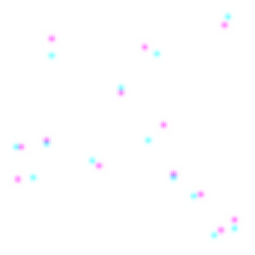
There are two kinds of particles, turquoise and pink, and they seem to be attracted to each other. They are close together. This happens quite often, by way of chemical interaction between the molecules. But not always:

In this picture, it looks like the two kinds don't care for each other at all - they aren't particularly close to each other; uncorrelated. We might conclude there isn't any chemical interaction between them.
We want to quantify this notion of a correlation between two kinds of particles to have a statistical test - like Pearson's $\chi^2$-test - but taking in these microscopic images. The thing is that, at small scales, microscopes tend to produce blurry images:
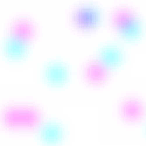
Let's first try to work with these blurry images. We get an image (width $w$ and height $h$ in pixels) with two different channels representing the signal strength from both molecule types. For this, we need a number representing the correlation. So our correlation is a function
$$f : \mathbb R^{w \times h \times 2} \to [-1, 1] $$
where a correlation of 0 means a completely random distribution, 1 means exact alignment and -1 exact avoidance. Now we can treat each pixel as an observation of two random variables, the strength of the signal from each molecule, and run standard statistical correlation tests like the one mentioned above.
A Simulation
Let's simulate the situation. We generate a pink point cloud of $n$ molecules by putting it randomly in the unit square. We then embed them into a bitmap by placing a gaussian distribution with standard deviation $b$ at the nearest pixel of the point. The $b$ stands for the blurriness of the microscope.
Then, we can add another normal distribution to the pink point cloud to get the blue point cloud. This second Gaussian is centered and has standard deviation $\sigma$. The larger $\sigma$, the more 'uncorrelated' the two point clouds.
We can also draw a line between corresponding blue and pink molecules, to see how far off they landed.
import sys
try:
    if "pyodide" in sys.modules:
        import piplite
        await piplite.install('ipywidgets == 7.7')
except:
    print("piplite not found, ignore this if you are not using Jupyterlite")
import scipy
import numpy as np
import matplotlib.colors as colors
import matplotlib.pyplot as plt
from ipywidgets import interact, interactive, fixed, interact_manual, FloatSlider, BoundedIntText, IntSlider, Checkbox, widgets
from IPython.display import display
from scipy.ndimage import gaussian_filter
def show_correlation(n, blur_dist, corr, show_connection = False, seed=0, plot=True):
    """
    Input:
        n - an integer, the number of blue and pink dots each
        blur_dist - a positive float, how much the bitmaps are blurred
        corr - a positive float, the standard deviation of the offset between blue and pink points
        show_connection - a boolean, whether or not to show connections between corresponding pink and blue dots

    Output:
        A float, the computed correlation
    """

    # Resolution of bitmap
    res = 256

    # Setting a seed for reproducability between
    # different paramters
    np.random.seed(seed)

    # Generating point clouds
    p1 = np.random.random((n,2))

    # We simulate an actual correlation of the second particle
    # type by adding a Gaussian to the first.

    p2 = p1 + np.random.normal(0, corr, (n,2))

    # Since we only consider a finite area, we wrap around
    # particles off the square

    for p in p2:
        p[0] = p[0] % 1
        p[1] = p[1] % 1

    # Conversion into bitmaps
    bm1 = np.zeros((res,res))
    bm2 = np.zeros((res,res))

    bm1[(p1 * res).astype(int)[:,0], (p1 * res).astype(int)[:,1]] = 1
    bm2[(p2 * res).astype(int)[:,0], (p2 * res).astype(int)[:,1]] = 1

    # Blurring the bitmaps
    bm1_blur = gaussian_filter(bm1, blur_dist * res, mode = 'wrap')
    bm2_blur = gaussian_filter(bm2, blur_dist * res, mode = 'wrap')


    # The calculated correlation coefficient
    ccc = np.corrcoef(np.vstack((bm1_blur.ravel(), bm2_blur.ravel())))[1,0]

    # Plotting (in red + green channels)
    bm1_blur = np.maximum(1 - 700 * blur_dist * (bm1_blur / np.linalg.norm(bm1_blur)), 0)
    bm2_blur = np.maximum(1 - 700 * blur_dist * (bm2_blur / np.linalg.norm(bm2_blur)), 0)

    mixed_image = np.stack((bm1_blur, bm2_blur, np.ones((res,res))), 2)

    if plot:
        fig = plt.figure(figsize=(20,20))

        plt.title("Computed Correlation Coefficient: {}".format(np.round(ccc, 4)), fontsize=20)
        plt.xticks([0, (res-1)/2 ,res-1], ["0", "0.5", "1"], fontsize=20)
        plt.yticks([0, (res-1)/2, res-1], ["0", "0.5", "1"], fontsize=20)
        plt.axis('off')

        if show_connection:
            # Show lines between the two associated points

            p1 *= res
            p2 *= res

            for i in range(n):
                plt.plot([p1[i][1], p2[i][1]], [p1[i][0], p2[i][0]], color='cornflowerblue', marker='')

        plt.imshow(mixed_image / np.max(mixed_image))
        plt.show()
    return ccc


# Creating widgets for interactive Visualization
n_widget = IntSlider(description='$n$',
                     min=2, max=20, value=8,
                     continuous_update=False)
blur_widget = FloatSlider(description='$b$',
                          min=0.005, max=0.16,
                          step=0.01, value=0.05,
                          continuous_update=True)
corr_widget = FloatSlider(description='$\sigma$',
                          min=0, max=0.3,
                          step=0.01, value=0.1,
                          continuous_update=False)
connection_widget = Checkbox(description="Show Connections",
                             value = False)
seed_widget = BoundedIntText(description='Seed',
                             value=1,min=0)

ui = widgets.VBox([n_widget, blur_widget, corr_widget, connection_widget, seed_widget])
widget = interactive(show_correlation, n=10, blur_dist=0.04, corr=0.1, seed=0)
out = widgets.interactive_output(show_correlation, {'n': n_widget, 'blur_dist': blur_widget, 'corr':corr_widget, 'show_connection':connection_widget, 'seed':seed_widget})

display(ui, out)
The Problem with Pointwise Correlation
Notice anything in particular? There are a lot of things to discuss here, but how about this: The correlation coefficient is very much dependent on the blur, which can be fatal in practice. Let us further investigate this by plotting the correlation as a function of the blurriness. Again, $n$ is the number of particles for each type and $\sigma$ is the standard deviation for the distance between the two types.
# Creating widgets for interactive Visualization
n_widget = IntSlider(description='$n$',
                     min=2, max=20, value=8,
                     continuous_update=False)
corr_widget = FloatSlider(description='$\sigma$',
                          min=0, max=0.3,
                          step=0.01, value=0.1,
                          continuous_update=False)

ui = widgets.VBox([n_widget, corr_widget])


def plot_correlation(n, corr):
    fig, ax = plt.subplots()
    CCCs = []
    blurs = np.linspace(0, 0.1, num=20)

    for blur in blurs:
        CCCs.append(show_correlation(n, blur, corr, plot=False))

    ax.plot(blurs, CCCs, color=colors.hsv_to_rgb([0.03*n, 0.05*n, 0.5 + 0.02*n]))

    plt.xlabel('Blur Coefficient $b$')
    plt.ylabel('Calculated Correlation Coefficient')
    plt.title("Calculated Correlation for different Blurrinesses $b$ and number of Molecules $n$")
    plt.show()

widget = interactive(plot_correlation, n=10, corr=0.1)
out = widgets.interactive_output(plot_correlation, {'n': n_widget, 'corr':corr_widget})

display(ui, out)
And once more for many different numbers of points at once:
ui = widgets.VBox([corr_widget])


def plot_correlation_2(corr):
    fig, ax = plt.subplots()
    for n in range(1, 20):
        CCCs = []
        blurs = np.linspace(0, 0.1, num=20)

        for blur in blurs:
            CCCs.append(show_correlation(n, blur, corr, plot=False))


        ax.plot(blurs, CCCs, color=colors.hsv_to_rgb([0.03*n, 0.05*n, 0.5 + 0.02*n]), label='$n$ = '+str(n))

    ax.legend(bbox_to_anchor=(1, 1),
          bbox_transform=fig.transFigure)
    plt.xlabel('Blur Coefficient $b$')
    plt.ylabel('Calculated Correlation Coefficient')
    plt.show()

widget = interactive(plot_correlation, n=10, corr=0.1)
out = widgets.interactive_output(plot_correlation_2, {'corr':corr_widget})

display(ui, out)
And it looks like especially for low blurs, this pixel-wise method is not useful at all. No matter what value $\sigma$ takes, the Correlation Coefficient is near 0. This is especially frustrating, because for good microscopes, i. e. low blur, we should get more accurate information about the particles' correlation, too.
So, is there another way to look at the problem?
Optimal Transport to the Rescue
If microscopes become really good, we can move away from this pixel-based approach and look at the molecules as points in continuous space. The question then becomes: When are two point clouds close together?
This is where at we will consider in the next notebook in this series, using optimal transport theory!
Written by Thilo Stier and Lennart Finke. Published under the MIT license.